easyCHEM tutorial#
You can find an executable version (but without the comparison to petitRADTRANS, since that needs a pRT install) of this notebook on Google Colab here.
We begin by loading the relevant packages: numpy, matplotlib, and easychem itself.
[1]:
import matplotlib.pyplot as plt
import numpy as np

import easychem.easychem as ec

plt.rcParams['figure.figsize'] = (10, 6)
Chemistry is calculated by creating objects from easychem’s ExoAtmos class.
[2]:
exo = ec.ExoAtmos()
By default, easychem assumes solar atmospheric abundances, following Asplund et al. (2009). You can switch to any other composition, however, and then update the abundances using exo.updateAtomAbund(), see an example further below.
The reactant species which are added by default, and are a reasonable selection for gas-dominated atmospheres, are
'H', 'H2', 'He', 'O', 'C', 'N', 'Mg', 'Si', 'Fe', 'S', 'Al', 'Ca', 'Na', 'Ni', 'P', 'K', 'Ti', 'CO', 'OH', 'SH', 'N2', 'O2', 'SiO', 'TiO', 'SiS', 'H2O', 'C2', 'CH', 'CN', 'CS', 'SiC', 'NH', 'SiH', 'NO', 'SN', 'SiN', 'SO', 'S2', 'C2H', 'HCN', 'C2H2,acetylene', 'CH4', 'AlH', 'AlOH', 'Al2O', 'CaOH', 'MgH', 'MgOH', 'PH3', 'CO2', 'TiO2', 'Si2C', 'SiO2', 'FeO', 'NH2', 'NH3', 'CH2', 'CH3', 'H2S', 'VO', 'VO2', 'NaCl', 'KCl', 'FeH', 'e-', 'H+', 'H-', 'Na+', 'K+', 'PH2', 'P2', 'PS', 'PO', 'P4O6', 'PH', 'V', 'VO(c)','VO(L)','MgSiO3(c)','SiC(c)', 'Fe(c)','Al2O3(c)','Na2S(c)','KCl(c)','Fe(L)','SiC(L)', 'MgSiO3(L)','H2O(L)','H2O(c)','TiO(c)','TiO(L)', 'TiO2(c)','TiO2(L)','H3PO4(c)','H3PO4(L)'.
More species (molecular, ions, condensates, etc.) can be added if they have a corresponding entry in easychem’s thermo_easy_chem_simp_own.inp file.
If you want to print the reactants that are available in thermo_easy_chem_simp_own you can do so like this:
[3]:
exo.print_available_species()
1: H
2: H2
3: He
4: O
5: C
6: N
7: Mg
8: Si
9: Fe
10: S
11: AL
12: Ca
13: Na
14: Ni
15: P
16: K
17: Ti
18: CO
19: OH
20: SH
21: N2
22: O2
23: SiO
24: TiO
25: SiS
26: H2O
27: C2
28: CH
29: CN
30: CS
31: SiC
32: NH
33: SiH
34: NO
35: SN
36: SiN
37: SO
38: S2
39: C2H
40: HCN
41: C2H2,acetylene
42: CH4
43: ALH
44: ALOH
45: AL2O
46: CaOH
47: MgH
48: MgOH
49: PH3
50: CO2
51: TiO2
52: Si2C
53: SiO2
54: FeO
55: NH2
56: NH3
57: CH2
58: CH3
59: H2S
60: V
61: VO
62: VO2
63: NaCL
64: KCL
65: MgSiO3(c)
66: Mg2SiO4(c)
67: SiC(c)
68: Fe(c)
69: AL2O3(c)
70: Na2S(c)
71: KCL(c)
72: e-
73: H+
74: H-
75: Na+
76: K+
77: H2O(c)
78: TiO(c)
79: VO(c)
80: NaOH
81: KOH
82: Fe(L)
83: Mg2SiO4(L)
84: SiC(L)
85: MgSiO3(L)
86: H2O(L)
87: TiO(L)
88: VO(L)
89: NaAlSi3O8(c)
90: KAlSi3O8(c)
91: MgAl2O4(c)
92: FeO(c)
93: Fe2O3(c)
94: Fe3O4(c)
95: CaMgSi2O6(c)
96: Fe2SiO4(c)
97: PH2
98: P2
99: PS
100: PO
101: P4O6
102: PH
103: TiO2(c)
104: TiO2(L)
105: H3PO4(L)
106: H3PO4(c)
107: H3PO4
108: HCL
109: SiH4
110: NH4CL(c)
111: SiO2(c)
112: Fe+
113: He+
114: Ca+
115: FeH
The thermo_easy_chem_simp_own.inp file follows the typical CEA input data file structure (NASA polynomials), so you can add more species if you have the corresponding thermodynamic data. The easiest is to access the NASA Glenn thermodynamic database, by using their Thermo Build tool. You then need to add the polynomial cofficients to the thermo_easy_chem_simp_own.inp file (how to access it is described below). Make sure not to add any extra
spaces, etc., to the data in the copying process, as this will lead to errors.
Next we show how to construct the standard path of thermo_easy_chem_simp_own.inp, so you can modify it. You can also create a local copy elsewhere, and then reference to it when creating the ExoAtmos object as exo = ec.ExoAtmos(thermofpath='path_to_your_file'). This may be preferable if you add many new species, because updating the easyCHEM package will overwrite the default thermo_easy_chem_simp_own.inp file.
[4]:
thermo_file_path = ec.__file__.replace('easychem.py','thermo_easy_chem_simp_own.inp')
This is what the first few lines of the default file look like, copied from the CEA input data file. This is for the species H, so atomic hydrogen.
[5]:
# show the first few lines:
f = open(thermo_file_path, 'r')
lines = f.readlines()
f.close()

for i in range(14):
    print(lines[i][:-1])
H                 D0(H2):Herzberg,1970. Moore,1972. Gordon,1999.
 4 g 6/97 H   1.00    0.00    0.00    0.00    0.00 0    1.0079400     217998.828
     60.000    300.0007 -2.0 -1.0  0.0  1.0  2.0  3.0  4.0  0.0         6197.428
  0.00000000D+00  0.00000000D+00  0.25000000D+01  0.00000000D+00  0.00000000D+00
  0.00000000D+00  0.00000000D+00  0.00000000D+00  0.25473708D+05 -0.44668285D+00
    300.000   1000.0007 -2.0 -1.0  0.0  1.0  2.0  3.0  4.0  0.0         6197.428
 0.000000000D+00 0.000000000D+00 2.500000000D+00 0.000000000D+00 0.000000000D+00
 0.000000000D+00 0.000000000D+00                 2.547370801D+04-4.466828530D-01
   1000.000   6000.0007 -2.0 -1.0  0.0  1.0  2.0  3.0  4.0  0.0         6197.428
 6.078774250D+01-1.819354417D-01 2.500211817D+00-1.226512864D-07 3.732876330D-11
-5.687744560D-15 3.410210197D-19                 2.547486398D+04-4.481917770D-01
   6000.000  20000.0007 -2.0 -1.0  0.0  1.0  2.0  3.0  4.0  0.0         6197.428
 2.173757694D+08-1.312035403D+05 3.399174200D+01-3.813999680D-03 2.432854837D-07
-7.694275540D-12 9.644105630D-17                 1.067638086D+06-2.742301051D+02
Calculating equilibrium abundances at single pressure-temperature point:#
This is how you would calculate the atmospheric composition at a single point in the atmosphere, in this case at 1 bar and 1000 K:
[6]:
%time exo.solve(1, 1000) # pressure = 1 bar; temperature = 1000 K
CPU times: user 9.36 ms, sys: 462 μs, total: 9.82 ms
Wall time: 9.87 ms
You can either get the result in the form of a numpy.ndarray, or a dictionary. Here first the arrays:
[7]:
print(exo.reacMass) # mass fractions
print(exo.reacMols) # number fractions (aka volume mixing ratios, VMRs)
[9.06021531e-10 7.37035941e-01 2.49582309e-01 7.14991122e-23
 1.71120160e-31 1.32997188e-23 1.32552621e-04 1.69366979e-38
 3.59250117e-13 1.75854880e-14 9.25083906e-26 1.02065922e-05
 2.49918731e-05 7.13609915e-05 8.04922752e-14 1.28500554e-06
 7.75264052e-30 1.47737546e-04 3.29252914e-14 1.44426843e-09
 6.73058823e-04 6.02815393e-26 5.03657385e-26 1.75359099e-23
 7.51800016e-27 5.00502873e-03 1.99056607e-37 1.58180608e-27
 1.36952561e-21 8.43062897e-15 0.00000000e+00 1.11254028e-19
 2.96316331e-36 4.90846764e-19 3.12107218e-18 1.55689889e-40
 6.04280952e-16 9.55662579e-13 1.79368225e-26 3.36098596e-09
 4.47393261e-13 3.07857565e-03 6.95996734e-24 2.84105593e-17
 9.34852935e-32 7.69568804e-05 3.94895382e-10 2.14643880e-07
 6.30982696e-06 2.52917559e-07 5.60594705e-22 0.00000000e+00
 8.42650914e-32 5.61152868e-20 7.99163549e-14 2.51643916e-05
 1.05201637e-19 1.25782953e-10 3.29138971e-04 1.11000627e-19
 1.28934650e-16 1.08724834e-05 3.40209843e-06 2.44241088e-18
 0.00000000e+00 1.41372724e-21 3.19478213e-16 1.73529394e-13
 3.81727879e-08 4.80369239e-08 1.62565617e-10 3.64336842e-11
 4.15672327e-32 3.43966910e-11 7.20735804e-23 6.97888442e-17
 4.17410293e-07 0.00000000e+00 2.37988650e-03 0.00000000e+00
 1.29376650e-03 1.05261688e-04 0.00000000e+00 0.00000000e+00
 0.00000000e+00 0.00000000e+00 0.00000000e+00 0.00000000e+00
 0.00000000e+00 0.00000000e+00 0.00000000e+00 5.21473752e-06
 0.00000000e+00 0.00000000e+00 0.00000000e+00]
[2.09757275e-09 8.53173161e-01 1.45501532e-01 1.04278053e-23
 3.32451900e-32 2.21565731e-24 1.27259043e-05 1.40715695e-39
 1.50109640e-14 1.27973232e-15 8.00038699e-27 5.94252040e-07
 2.53665534e-06 2.83705377e-06 6.06395085e-15 7.66907676e-08
 3.77928285e-31 1.23075662e-05 4.51741733e-15 1.01899393e-10
 5.60638811e-05 4.39588782e-27 2.66588435e-27 6.40695729e-25
 2.91648031e-28 6.48281228e-04 1.93363385e-38 2.83520794e-28
 1.22829369e-22 4.46330657e-16 0.00000000e+00 1.72901172e-20
 2.37660534e-37 3.81708947e-20 1.58075853e-19 8.63087334e-42
 2.93367053e-17 3.47727710e-14 1.67221751e-27 2.90196476e-10
 4.00950832e-14 4.47794913e-04 5.80242549e-25 1.50707071e-18
 3.11798884e-33 3.14571321e-06 3.64029108e-11 1.21236976e-08
 4.33078303e-07 1.34099916e-08 1.63788763e-23 0.00000000e+00
 3.27252257e-33 1.82257003e-21 1.16386162e-14 3.44792290e-06
 1.75012529e-20 1.95223298e-11 2.25354111e-05 3.86927722e-21
 3.62743803e-18 4.34104653e-07 1.06484798e-07 1.03890249e-14
 0.00000000e+00 3.27120550e-21 3.24275595e-17 1.03566006e-14
 2.70005610e-09 1.80945032e-09 6.01750860e-12 1.80987634e-12
 4.41101397e-34 2.50963799e-12 3.30141658e-24 2.86437149e-18
 1.45501532e-08 0.00000000e+00 5.53181153e-05 0.00000000e+00
 5.40589451e-05 2.40896978e-06 0.00000000e+00 0.00000000e+00
 0.00000000e+00 0.00000000e+00 0.00000000e+00 0.00000000e+00
 0.00000000e+00 0.00000000e+00 0.00000000e+00 1.52358808e-07
 0.00000000e+00 0.00000000e+00 0.00000000e+00]
And here as dictionaries:
[8]:
print(exo.result_mass()) # mass fractions
print(exo.result_mol())  # number fractions (VMRs)
{'H': 9.060215311210445e-10, 'H2': 0.7370359414025471, 'He': 0.24958230903837048, 'O': 7.149911217544124e-23, 'C': 1.7112016049400616e-31, 'N': 1.3299718750399277e-23, 'Mg': 0.00013255262131788516, 'Si': 1.6936697908725963e-38, 'Fe': 3.592501171731354e-13, 'S': 1.758548799255385e-14, 'Al': 9.250839059180737e-26, 'Ca': 1.0206592198518813e-05, 'Na': 2.4991873135602487e-05, 'Ni': 7.136099148215103e-05, 'P': 8.049227516154347e-14, 'K': 1.2850055396780097e-06, 'Ti': 7.752640516106653e-30, 'CO': 0.00014773754629475287, 'OH': 3.29252913681285e-14, 'SH': 1.444268425252039e-09, 'N2': 0.0006730588234471623, 'O2': 6.028153927044227e-26, 'SiO': 5.036573850291348e-26, 'TiO': 1.753590994404444e-23, 'SiS': 7.518000160799364e-27, 'H2O': 0.0050050287286896354, 'C2': 1.9905660674537797e-37, 'CH': 1.5818060812799341e-27, 'CN': 1.3695256054855985e-21, 'CS': 8.430628971769065e-15, 'SiC': 0.0, 'NH': 1.112540284838103e-19, 'SiH': 2.9631633121978255e-36, 'NO': 4.908467642959679e-19, 'SN': 3.1210721788627002e-18, 'SiN': 1.556898890113162e-40, 'SO': 6.042809518892262e-16, 'S2': 9.556625791632257e-13, 'C2H': 1.793682248708611e-26, 'HCN': 3.3609859642060986e-09, 'C2H2,acetylene': 4.473932611934447e-13, 'CH4': 0.00307857564546318, 'AlH': 6.9599673407287e-24, 'AlOH': 2.841055932011771e-17, 'Al2O': 9.348529351337869e-32, 'CaOH': 7.695688035779128e-05, 'MgH': 3.9489538236908906e-10, 'MgOH': 2.1464388005387652e-07, 'PH3': 6.3098269565836405e-06, 'CO2': 2.529175589451864e-07, 'TiO2': 5.605947045035003e-22, 'Si2C': 0.0, 'SiO2': 8.426509141720605e-32, 'FeO': 5.611528681357326e-20, 'NH2': 7.991635487256614e-14, 'NH3': 2.5164391604819862e-05, 'CH2': 1.0520163700313678e-19, 'CH3': 1.2578295319786506e-10, 'H2S': 0.0003291389708913377, 'VO': 1.110006274332286e-19, 'VO2': 1.2893464956699093e-16, 'NaCl': 1.0872483391224454e-05, 'KCl': 3.4020984302171102e-06, 'e-': 2.4424108814376297e-18, 'H+': 0.0, 'H-': 1.413727240842205e-21, 'Na+': 3.194782126370684e-16, 'K+': 1.735293941671396e-13, 'PH2': 3.8172787859280013e-08, 'P2': 4.8036923911918054e-08, 'PS': 1.6256561723676123e-10, 'PO': 3.6433684245908263e-11, 'P4O6': 4.156723271256555e-32, 'PH': 3.439669101084069e-11, 'V': 7.207358037896342e-23, 'FeH': 6.978884422441204e-17, 'VO(c)': 4.1741029303091954e-07, 'VO(L)': 0.0, 'MgSiO3(c)': 0.0023798865026623253, 'SiC(c)': 0.0, 'Fe(c)': 0.0012937665026635675, 'Al2O3(c)': 0.0001052616880830774, 'Na2S(c)': 0.0, 'KCl(c)': 0.0, 'Fe(L)': 0.0, 'SiC(L)': 0.0, 'MgSiO3(L)': 0.0, 'H2O(L)': 0.0, 'H2O(c)': 0.0, 'TiO(c)': 0.0, 'TiO(L)': 0.0, 'TiO2(c)': 5.214737522133029e-06, 'TiO2(L)': 0.0, 'H3PO4(c)': 0.0, 'H3PO4(L)': 0.0}
{'H': 2.0975727520751938e-09, 'H2': 0.8531731613889914, 'He': 0.1455015322134447, 'O': 1.0427805262558948e-23, 'C': 3.3245189966704667e-32, 'N': 2.2156573075377306e-24, 'Mg': 1.2725904348700085e-05, 'Si': 1.4071569525419348e-39, 'Fe': 1.5010963972285114e-14, 'S': 1.2797323236340855e-15, 'Al': 8.000386987869187e-27, 'Ca': 5.942520402868172e-07, 'Na': 2.5366553408844942e-06, 'Ni': 2.837053768754872e-06, 'P': 6.063950853722436e-15, 'K': 7.669076761340257e-08, 'Ti': 3.779282847834336e-31, 'CO': 1.2307566240225606e-05, 'OH': 4.517417332161247e-15, 'SH': 1.0189939334539693e-10, 'N2': 5.606388106999189e-05, 'O2': 4.3958878181384396e-27, 'SiO': 2.6658843536105366e-27, 'TiO': 6.406957294704535e-25, 'SiS': 2.9164803073796157e-28, 'H2O': 0.0006482812281051972, 'C2': 1.933633853040219e-38, 'CH': 2.8352079429267937e-28, 'CN': 1.2282936932382365e-22, 'CS': 4.463306565002933e-16, 'SiC': 0.0, 'NH': 1.729011724722473e-20, 'SiH': 2.376605343795006e-37, 'NO': 3.81708946943682e-20, 'SN': 1.580758530891181e-19, 'SiN': 8.630873338226105e-42, 'SO': 2.9336705341769884e-17, 'S2': 3.477277097913191e-14, 'C2H': 1.6722175066316983e-27, 'HCN': 2.901964762255783e-10, 'C2H2,acetylene': 4.0095083169777504e-14, 'CH4': 0.0004477949125049742, 'AlH': 5.802425491326337e-25, 'AlOH': 1.5070707068818614e-18, 'Al2O': 3.117988838335988e-33, 'CaOH': 3.1457132080886685e-06, 'MgH': 3.640291079382753e-11, 'MgOH': 1.2123697604533374e-08, 'PH3': 4.3307830276154646e-07, 'CO2': 1.3409991620322658e-08, 'TiO2': 1.637887634603503e-23, 'Si2C': 0.0, 'SiO2': 3.272522565047609e-33, 'FeO': 1.822570028822328e-21, 'NH2': 1.1638616171921802e-14, 'NH3': 3.44792290010055e-06, 'CH2': 1.750125292267798e-20, 'CH3': 1.9522329824263442e-11, 'H2S': 2.2535411131326076e-05, 'VO': 3.8692772161265396e-21, 'VO2': 3.6274380293958e-18, 'NaCl': 4.3410465270167176e-07, 'KCl': 1.0648479840952357e-07, 'e-': 1.0389024907501902e-14, 'H+': 0.0, 'H-': 3.2712054951993645e-21, 'Na+': 3.242755948487474e-17, 'K+': 1.0356600619222612e-14, 'PH2': 2.7000561045011615e-09, 'P2': 1.8094503179420968e-09, 'PS': 6.017508596579774e-12, 'PO': 1.8098763395497807e-12, 'P4O6': 4.4110139669765035e-34, 'PH': 2.5096379869908916e-12, 'V': 3.3014165760177575e-24, 'FeH': 2.864371493950719e-18, 'VO(c)': 1.4550153219384042e-08, 'VO(L)': 0.0, 'MgSiO3(c)': 5.5318115285960785e-05, 'SiC(c)': 0.0, 'Fe(c)': 5.405894509610587e-05, 'Al2O3(c)': 2.408969779611065e-06, 'Na2S(c)': 0.0, 'KCl(c)': 0.0, 'Fe(L)': 0.0, 'SiC(L)': 0.0, 'MgSiO3(L)': 0.0, 'H2O(L)': 0.0, 'H2O(c)': 0.0, 'TiO(c)': 0.0, 'TiO(L)': 0.0, 'TiO2(c)': 1.5235880818334183e-07, 'TiO2(L)': 0.0, 'H3PO4(c)': 0.0, 'H3PO4(L)': 0.0}
Calculating equilibrium abundances for a whole atmospheric P-T structure:#
Let’s assume an isothermal (1000 K) atmospheric temperature structure (100 layers) going from 1 µbar to 100 bar (equidistantly log-spaced). We can then calculate the atmospheric structure as follows:
[9]:
press = np.logspace(-6,2,100)
temp = np.ones(100) * 1000.

%time exo.solve(press, temp)
CPU times: user 276 ms, sys: 15 ms, total: 291 ms
Wall time: 291 ms
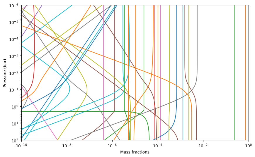
We can plot the results as follows. We will not show the legend here, because there are too many species… Adding a legend makes more sense if you only plot those species you are interested in.
[10]:
mass_fractions = exo.result_mass()
for spec in exo.reactants:
    plt.loglog(mass_fractions[spec], press, label = spec)

plt.ylim([1e2,1e-6])
plt.xlim([1e-10, 1])

plt.xlabel('Mass fractions')
plt.ylabel('Pressure (bar)')
[10]:
Text(0, 0.5, 'Pressure (bar)')
Changing metallicity#
In the following example, we are changing the considered atmosphere’s metallicity. The elemental composition exo.atomAbunds will then automatically be updated with the new value of exo.metallicity taken into account. exo.metallicity is defined with respect to solar, so if you change it all elemental abundances (except H and He) are scaled by 10**exo.metallicity (a value of 0 is thus solar).
[11]:
exo.metallicity = 0.5

%time exo.solve(press, temp)
mass_fractions = exo.result_mass()
CPU times: user 284 ms, sys: 14 ms, total: 298 ms
Wall time: 299 ms
Sanity check: let’s compare to the chemical equilibrium interpolation of petitRADTRANS:
[12]:
from petitRADTRANS.chemistry.pre_calculated_chemistry import PreCalculatedEquilibriumChemistryTable
chem = PreCalculatedEquilibriumChemistryTable()
[13]:
COs = 0.55 * np.ones_like(press) # solar
FeHs = 0.5 * np.ones_like(press) # metals are scaled by 10^0.5 * solar

pRT_mass_fractions, mean_molar_mass, nabla_ad = chem.interpolate_mass_fractions(
    COs,
    FeHs,
    temp,
    press,
    full=True)
Loading chemical equilibrium chemistry table from file '/Users/molliere/Documents/program_data/pRT3/input_data/pre_calculated_chemistry/equilibrium_chemistry/equilibrium_chemistry.chemtable.petitRADTRANS.h5'... Done.
Now we plot and compare the two resulting compositions:
[14]:
for i_spec, spec in enumerate(pRT_mass_fractions.keys()):

    plt.loglog(pRT_mass_fractions[spec],
               press,
               label = spec,
               linestyle = '-',
               color = 'C'+str(i_spec))
    try:
        plt.loglog(mass_fractions[spec],
                   press,
                   linestyle = ':',
                   color = 'C'+str(i_spec))
    except KeyError:
        pass

plt.ylim([1e2,1e-6])
plt.xlim([1e-10, 1])

plt.xlabel('Mass fractions')
plt.ylabel('Pressure (bar)')
plt.title('Solid = pRT chemistry interpolation, dashed = easyCHEM')
plt.legend()
[14]:
<matplotlib.legend.Legend at 0x121dc3850>
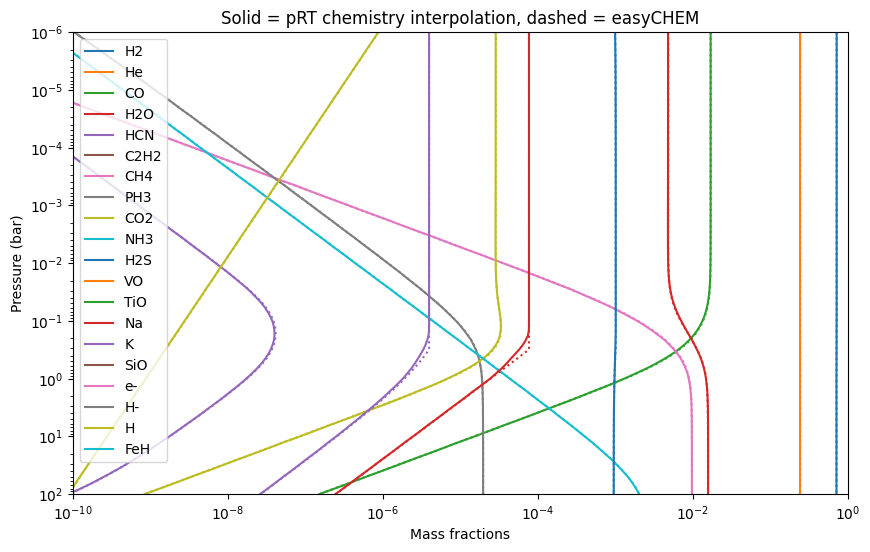
Note that there are slight differences, because pRT interpolates in an equilibrium abundance table, while easychem calculates the abundances at every P-T point from scratch. So differences are due to the interpolation effects in pRT, while easyCHEM is more accurate.
Changing C/O#
Next we change the carbon-to-oxygen number ratio. In easyCHEM this is done by changing the oxygen content of the atmosphere. You can also change carbon instead, however, see below.
C/O changing convention in easyCHEM: the C/O is changed by setting the oxygen abundance to carbon abundance/(C/O). This means that this operation will change the overall atmospheric metallicity, since only the oxygen abundance changes, while all other metal abundances remain the same (but note that all atom abundances, including H/He are normalized to sum to unity after any update step of the atom abundances). To exercise a finer control over the composition, the use of
updateAtomAbunds() is recommended (see an example for its use below), which allows the user to set the abundances of all elements independently. In that case users may renormalize the metal abundances after changing the oxygen (or carbon) abundance for an updated C/O ratio. Options could include conserving the metal atom mass or number, in comparison to H/He.
[15]:
exo.co = 1.2

%time exo.solve(press, temp)
mass_fractions = exo.result_mass()
CPU times: user 355 ms, sys: 14.7 ms, total: 370 ms
Wall time: 309 ms
Again we compare to pRT here:
[16]:
COs = 1.2 * np.ones_like(press)
FeHs = 0.5 * np.ones_like(press)

pRT_mass_fractions, mean_molar_mass, nabla_ad = chem.interpolate_mass_fractions(
    COs,
    FeHs,
    temp,
    press,
    full=True)

for i_spec, spec in enumerate(pRT_mass_fractions.keys()):

    plt.loglog(pRT_mass_fractions[spec],
               press,
               label = spec,
               linestyle = '-',
               color = 'C'+str(i_spec))
    try:
        plt.loglog(mass_fractions[spec],
                   press,
                   linestyle = ':',
                   color = 'C'+str(i_spec))
    except KeyError:
        pass

plt.ylim([1e2,1e-6])
plt.xlim([1e-10, 1])

plt.xlabel('Mass fractions')
plt.ylabel('Pressure (bar)')
plt.title('Solid = pRT chemistry interpolation, dashed = easyCHEM')
plt.legend()
[16]:
<matplotlib.legend.Legend at 0x145a60f90>
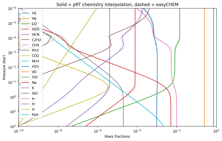
Again note the differences due to pRT’s interpolation.
Varying atmospheric elemental abundances freely#
This is an example for how to modify atmospheric elemental abundances freely. in this example we chose to allow the user to scale [C/H], [O/H] and [Fe/H] independently, where [X/H] is defined as \(\rm log_{10}(X/H)-log_{10}(X/H)_\odot\). “Fe” in this case stands for all elements except for C, H, O, He. Similar setups could also be used to implement atmospheric condensate rainout.
[17]:
# Start with a clean ExoAtmos object (so solar composition)
exo = ec.ExoAtmos()

# Copy the solar abundance setup
atom_abundances_solar = exo._atomAbunds.copy()

# Get atom names
atom_names = exo.atoms

# Implement function to return the modified abundances.
def update_atom_abundances(C_H, O_H, Fe_H):
  modif_abundances = atom_abundances_solar.copy()
  for i_spec, name in enumerate(atom_names):
    if name == 'C':
      modif_abundances[i_spec] = modif_abundances[i_spec]*10**C_H
    elif name == 'O':
      modif_abundances[i_spec] = modif_abundances[i_spec]*10**O_H
    elif name not in ['H', 'He', 'C', 'O']:
      modif_abundances[i_spec] = modif_abundances[i_spec]*10**Fe_H

  return modif_abundances
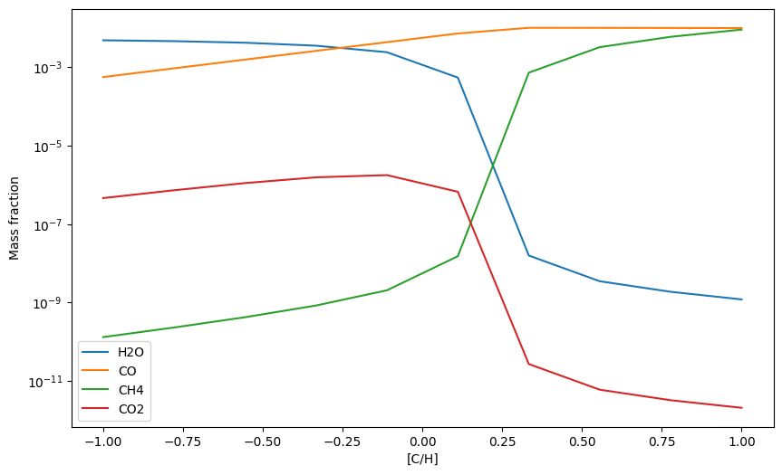
Let’s test how this setup behaves now! We start by changing [C/H] from -1 to 1.
[18]:
C_Hs = np.linspace(-1, 1, 10) # from 0.1 to 10 x solar

H2Os = np.zeros(10) # to store H2O mass fractions
COs = np.zeros(10)  # to store CO  mass fractions
CH4s = np.zeros(10) # to store CH4 mass fractions
CO2s = np.zeros(10) # to store CO2 mass fractions

for i, C_H in enumerate(C_Hs):
  update_abunds = update_atom_abundances(C_H,0,0) # make update abundance list
  exo.updateAtomAbunds(update_abunds) # update abundances
  exo.solve(0.001, 1200) # calculate composition at 1 mbar, 1200 K.
  mass_fractions = exo.result_mass()
  H2Os[i] = mass_fractions['H2O']
  COs[i] = mass_fractions['CO']
  CH4s[i] = mass_fractions['CH4']
  CO2s[i] = mass_fractions['CO2']

plt.plot(C_Hs, H2Os, label = 'H2O')
plt.plot(C_Hs, COs, label = 'CO')
plt.plot(C_Hs, CH4s, label = 'CH4')
plt.plot(C_Hs, CO2s, label = 'CO2')
plt.yscale('log')
plt.xlabel('[C/H]')
plt.ylabel('Mass fraction')
plt.legend()
plt.show()
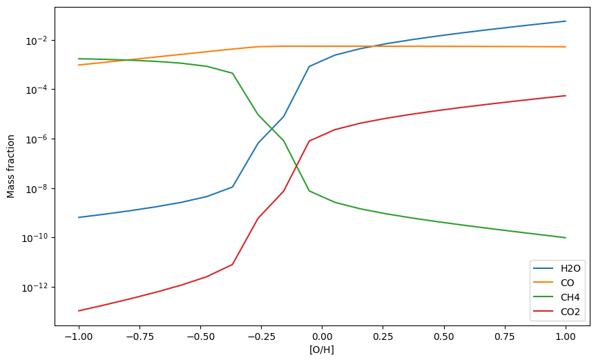
Now we change [O/H] from -1 to 1, then [Fe/H] from -1 to 1, then all three ([C/H], [O/H], [Fe/H]) at the same time.
[19]:
O_Hs = np.linspace(-1, 1, 20) # from 0.1 to 10 x solar
H2Os = np.zeros(20) # to store H2O mass fractions
COs = np.zeros(20) # to store CO mass fractions
CH4s = np.zeros(20) # to store CH4 mass fractions
CO2s = np.zeros(20) # to store CO2 mass fractions
for i, O_H in enumerate(O_Hs):
update_abunds = update_atom_abundances(0,O_H,0)
exo.updateAtomAbunds(update_abunds)
exo.solve(0.001, 1200)
mass_fractions = exo.result_mass()
H2Os[i] = mass_fractions['H2O']
COs[i] = mass_fractions['CO']
CH4s[i] = mass_fractions['CH4']
CO2s[i] = mass_fractions['CO2']
plt.plot(O_Hs, H2Os, label = 'H2O')
plt.plot(O_Hs, COs, label = 'CO')
plt.plot(O_Hs, CH4s, label = 'CH4')
plt.plot(O_Hs, CO2s, label = 'CO2')
plt.yscale('log')
plt.xlabel('[O/H]')
plt.ylabel('Mass fraction')
plt.legend()
plt.show()
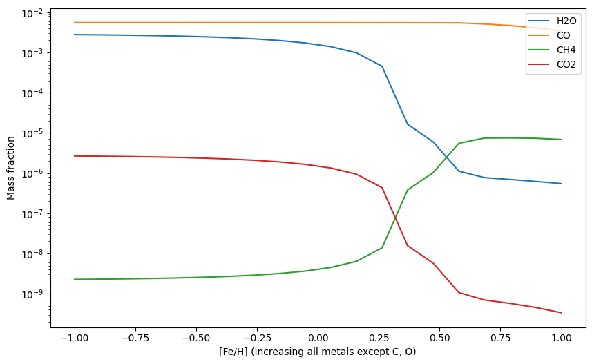
Fe_Hs = np.linspace(-1, 1, 20) # from 0.1 to 10 x solar
H2Os = np.zeros(20)
COs = np.zeros(20)
CH4s = np.zeros(20)
CO2s = np.zeros(20)
for i, Fe_H in enumerate(Fe_Hs):
update_abunds = update_atom_abundances(0,0,Fe_H)
exo.updateAtomAbunds(update_abunds)
exo.solve(0.001, 1200)
mass_fractions = exo.result_mass()
H2Os[i] = mass_fractions['H2O']
COs[i] = mass_fractions['CO']
CH4s[i] = mass_fractions['CH4']
CO2s[i] = mass_fractions['CO2']
plt.plot(Fe_Hs, H2Os, label = 'H2O')
plt.plot(Fe_Hs, COs, label = 'CO')
plt.plot(Fe_Hs, CH4s, label = 'CH4')
plt.plot(Fe_Hs, CO2s, label = 'CO2')
plt.yscale('log')
plt.xlabel('[Fe/H] (increasing all metals except C, O)')
plt.ylabel('Mass fraction')
plt.legend()
plt.show()
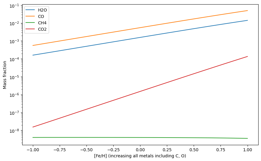
H2Os = np.zeros(20)
COs = np.zeros(20)
CH4s = np.zeros(20)
CO2s = np.zeros(20)
for i, Fe_H in enumerate(Fe_Hs):
update_abunds = update_atom_abundances(Fe_H,Fe_H,Fe_H)
exo.updateAtomAbunds(update_abunds)
exo.solve(0.001, 1200)
mass_fractions = exo.result_mass()
H2Os[i] = mass_fractions['H2O']
COs[i] = mass_fractions['CO']
CH4s[i] = mass_fractions['CH4']
CO2s[i] = mass_fractions['CO2']
plt.plot(Fe_Hs, H2Os, label = 'H2O')
plt.plot(Fe_Hs, COs, label = 'CO')
plt.plot(Fe_Hs, CH4s, label = 'CH4')
plt.plot(Fe_Hs, CO2s, label = 'CO2')
plt.yscale('log')
plt.xlabel('[Fe/H] (increasing all metals including C, O)')
plt.ylabel('Mass fraction')
plt.legend()
plt.show()
Ancillary outputs#
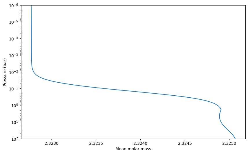
Mean molecular weight (aka mean molar mass)#
Can be accessed like this:
[20]:
exo = ec.ExoAtmos()

press = np.logspace(-6,2,100)
temp = np.ones(100) * 1000.

%time exo.solve(press, temp)
CPU times: user 500 ms, sys: 15.8 ms, total: 516 ms
Wall time: 296 ms
[21]:
plt.semilogy(exo.mmw, press)
plt.xlabel(r'Mean molar mass')
plt.ylim([100, 1e-6])
plt.ylabel('Pressure (bar)')
[21]:
Text(0, 0.5, 'Pressure (bar)')
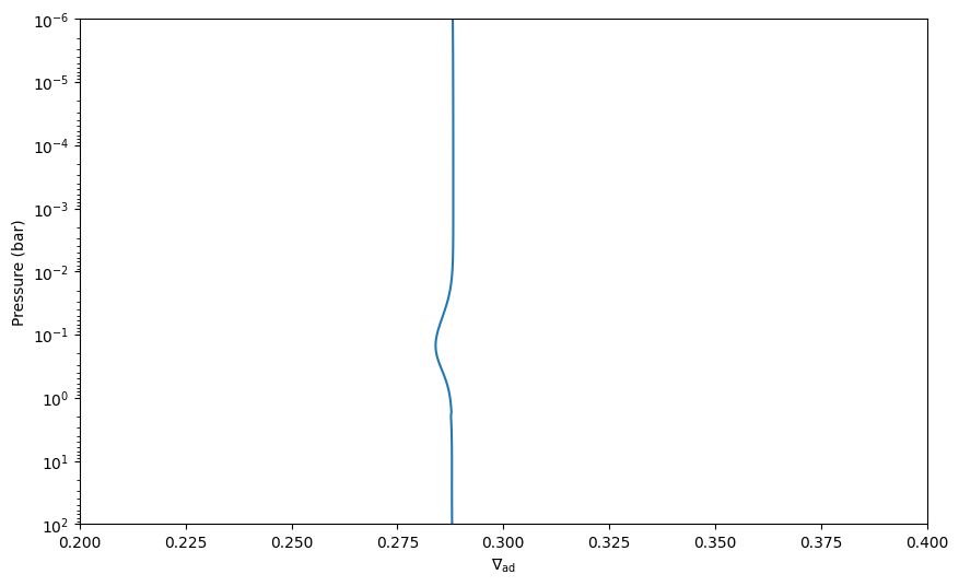
Adiabatic temperature gradient \(\nabla_{\rm ad}\)#
easyCHEM also outputs the atmosphere’s adiabatic temperature gradient, that is, \(\nabla_{\rm ad} = (d {\rm log T}/d {\rm log P})_{\rm ad}\). This is the gradient an atmosphere follows if it is convectively unstable. Note that easyCHEM is a CEA clone, so \(\nabla_{\rm ad}\) includes changes in chemical composition as the temperature is changed at a given pressure. \(\nabla_{\rm ad}\) therefore corresponds to the moist adiabatic lapse rate. Here an example for how to access \(\nabla_{\rm ad}\) in a solar composition atmosphere:
[22]:
nabla_ad = (exo.gamma2-1.)/exo.gamma2
plt.semilogy(nabla_ad, press)

plt.xlabel(r'$\nabla_{\rm ad}$')
plt.xlim([0.2, 0.4])
plt.ylim([100, 1e-6])
plt.ylabel('Pressure (bar)')
[22]:
Text(0, 0.5, 'Pressure (bar)')
Example calculation for a moist adiabat#
Below we set up an atmosphere that is inspired by Earth. That is, its atomic composition is mostly N and O, with traces of H. We start with a setup that contains only O2, O, N2, N and H2O as chemical reactants, that is, no condensibles (since we did not add H2O(L) or H2O(c), which would be liquid and icy water, respectively).
[23]:
atom_names = ['N', 'O', 'H']
atom_abundances = np.array([0.7, 0.3, 0.04]) # these are just ballpark relative number fractions
atom_abundances = atom_abundances/np.sum(atom_abundances) # normalizing here...
reactants = ['N2','O2', 'N', 'O', 'H2O']

earth = ec.ExoAtmos()
earth.atoms = atom_names
earth.updateAtomAbunds(atom_abundances)
earth.reactants = reactants

press = np.logspace(-6,0,100) # 1 microbar to 1 bar
temp = np.linspace(200,280,100) # Some nice habitable zone temperature
%time earth.solve(press, temp)
CPU times: user 37.8 ms, sys: 14.7 ms, total: 52.6 ms
Wall time: 17.5 ms
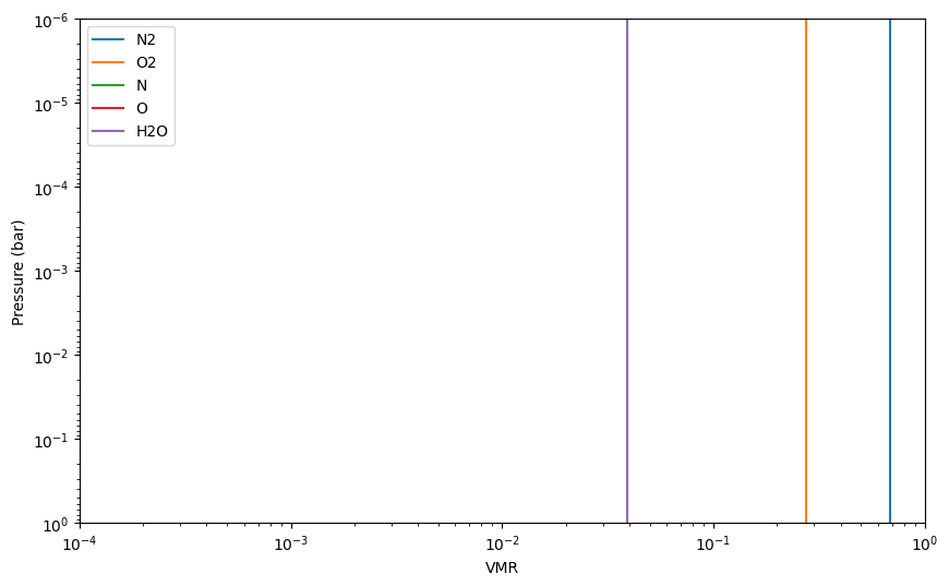
Let’s plot the resulting composition and store the adiabatic temperature gradient:
[24]:
mol_fractions = earth.result_mol()
for spec in earth.reactants:
    plt.loglog(mol_fractions[spec], press, label = spec)

plt.ylim([1e0,1e-6])
plt.xlim([1e-4, 1])

plt.legend()
plt.xlabel('VMR')
plt.ylabel('Pressure (bar)')
plt.show()

nabla_ad_dry = (earth.gamma2-1.)/earth.gamma2
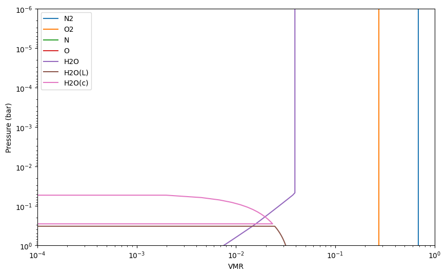
Now let’s do the same again, but add H2O(L) and H2O(c) to the reactants. This will allow us to see the effect of water condensation on the adiabatic temperature gradient.
[25]:
reactants = ['N2','O2', 'N', 'O', 'H2O', 'H2O(L)', 'H2O(c)']

earth.reactants = reactants

%time earth.solve(press, temp)

mol_fractions = earth.result_mol()
for spec in earth.reactants:
    plt.loglog(mol_fractions[spec], press, label = spec)

plt.ylim([1e0,1e-6])
plt.xlim([1e-4, 1])

plt.legend()
plt.xlabel('VMR')
plt.ylabel('Pressure (bar)')
plt.show()

nabla_ad_moist = (earth.gamma2-1.)/earth.gamma2
CPU times: user 40.3 ms, sys: 13.6 ms, total: 54 ms
Wall time: 17.5 ms
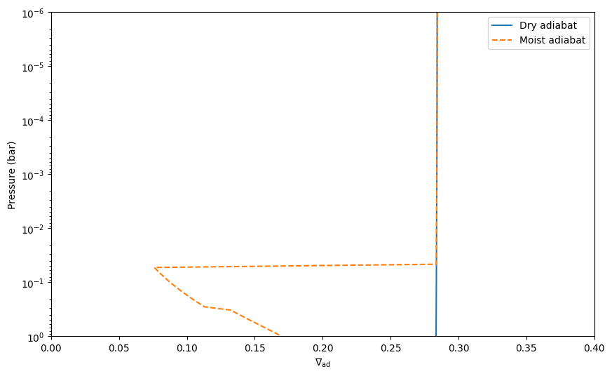
Now let’s plot the two adiabatic temperature gradients together, for the dry case (no water condensation) and the moist case (water condensation allowed):
[26]:
plt.semilogy(nabla_ad_dry, press, label = 'Dry adiabat')
plt.semilogy(nabla_ad_moist, press, label = 'Moist adiabat', linestyle = '--')
plt.xlabel(r'$\nabla_{\rm ad}$')
plt.ylabel('Pressure (bar)')
plt.ylim([1e0,1e-6])
plt.xlim([0., 0.4])
plt.legend()
plt.show()
Condensates: a word on stability#
Condensates are tricky to handle in any equilibrium chemistry code. This is because condensates cannot occur together if one can write down hypothetical reaction equations that transform them into each other while conserving the atom number. This only occurs if the formation of the involved condensates is thermodynamically favored (i.e., the temperature is cold enough and the pressure is high enough for the species to be stable). An example would be
For the Gibbs minimizer that is the backbone of easyCHEM the actual problem is that the matrix to be inverted becomes rank-deficient. easyCHEM’s standard selection is pretty stable against this problem, but things can still go bad in a retrieval when many different temperature - pressure combinations are tried. In this case easyCHEM will become very slow and give non-sensical solutions. What to do then is not entirely clear. The best thing likely is to check which species are expected to
condense at a given pressure, temperature and composition, and which of these dominate the mass budget, when compared to other species. A useful starting point are papers such as Visser et al. (2010). In general, always be weary of your results if easyCHEM prints SLOW ! to the terminal when running.